genrelessrecs

Final Report

Introduction

These days, we often hear the response “I listen to everything except country” when asked about a favorite genre of music. We are currently witnessing the rise of “genre-less music fans” [1], as online streaming services have greatly widened listeners’ tastes in music [2]. Exploring new genres is also beneficial, as research has shown that different genres have different abilities to provide relaxation, motivation, joy, and a stronger sense of self [3]. Many successful music recommendation systems are based on song genre [4], but recommendations based on social features [5] and lyrics [6] have been shown to perform just as well as audio-based recommendations. With an increase in listeners of many genres, does a recommendation system focused mainly on audio truly reflect the listeners’ interests?

Problem Definition

We propose an approach where we use features that aren’t strongly correlated to genre to predict music for users; this may include features such as lyrics and artist hotness. We call these features genreless features. With the increase in genreless music fans and the benefits of exploring new genres, we propose two models to assist in creating a song recommendation system:

1. Classify the genre of the input song
2. Recommend a new song with similar genreless features from a different genre

In completing these two goals, we can still provide a relevant recommendation while fostering the exploration of new genres.

Dataset Collection

We first collected all 1,000,000 track IDs and song IDs from the Million Song Dataset track_metadata.db file. From there, we were able to find the genre labels for 280,831 of these songs by using the tagtraum annotation for the Million Song Dataset. We then removed the songs from our dataset that did not contain genre labels.

To get the features for each song, we utilized the Spotify API. First, we had to find the Spotify IDs that corresponded to the track IDs and song IDs that we collected from the Million Song Dataset. We were able to do this using Acoustic Brainz Lab’s Million Song Dataset Echo Nest mapping archive. We were able to find corresponding Spotify IDs for 210,475 of our 280,831 datapoints. We then removed the songs which did not have a corresponding Spotify ID.

Once we had the Spotify IDs for each song in our dataset, we were able to use the Spotify API to retrieve the audio features pertaining to each of our 210,475 songs. These features include:

• danceability
• energy
• key
• loudness
• mode
• speechiness
• acousticness
• instrumentalness
• liveness
• valence
• tempo
• duration_ms
• time_signature

Dataset Exploration

Distribution of Genres

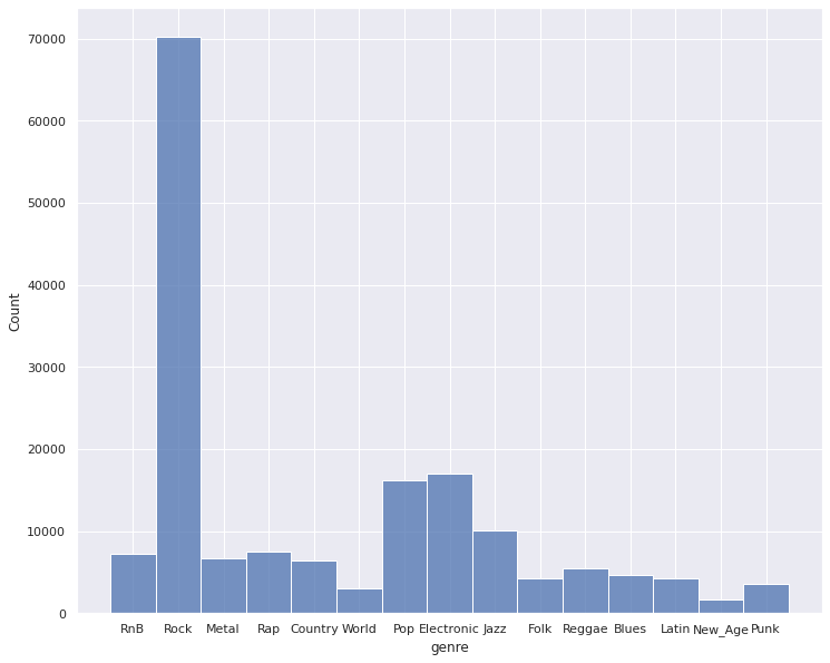
As determined from our review of existing works on the MSD dataset and the associated Tagtraum dataset, there is a high degree of data imbalance that we will need to address for our models. We will explore metrics measuring model “goodness” that takes this into account (metrics such as accuracy may not be a good behavior of a model exploring deeper relationships in the data. There are 15 unique categories that we have as genre labels with about 42% comprising of the category “Rock”. After the collection of our data, we retained 168,379 datapoints to train our models - losing points if not having an associated genre in the Tagtraum dataset or if not having a mapping from MSD Track ID to Spotify ID. The statistics presented throughout our exploration stage is on the 80 percent of data we use for training and cross validating (not the 20 percent held out for evaluation across models.

Feature Histograms

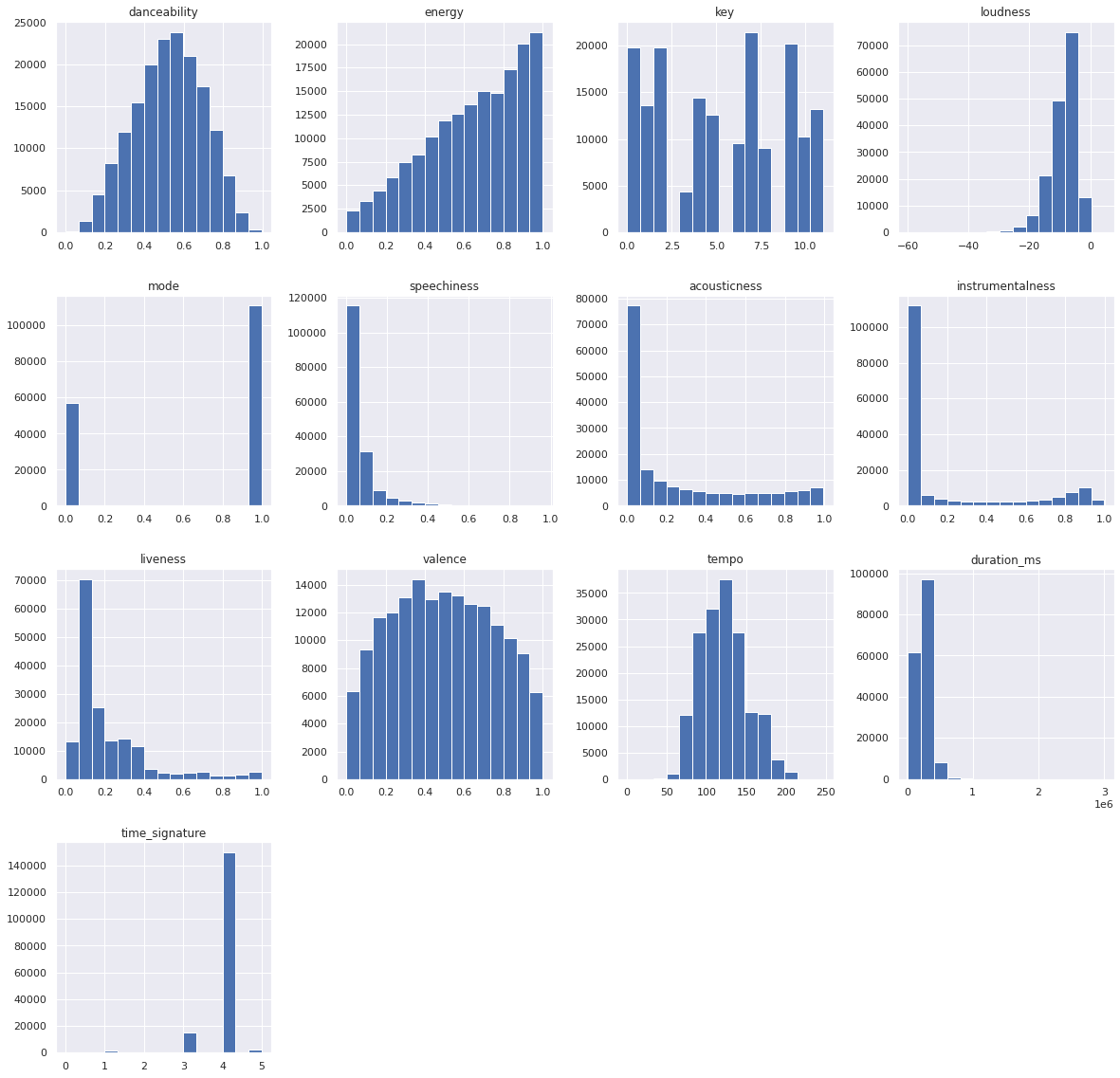
From the various historgrams, we can see initial need for data preprossing given the differences in ranges of values from feature to feature and difference in overall distributions.

Feature Correlation Heat Map

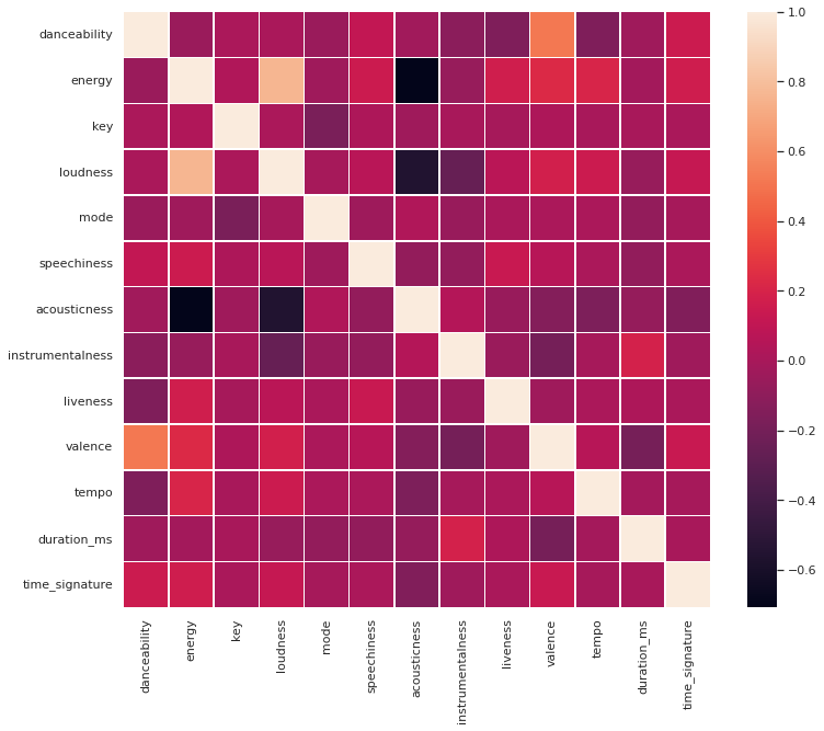
The above image explores the correlation between the features in our dataset. Intuitively we can see some of these relationships. For instance, accousticness which describes songs with less electric amplication is negativelely correlated with loudness and energy. Similarly, we can see how valance (how “happy” a song is) and danceability are positively correlated, and loudness and energy are positively correlated.

Features by Genre (Danceability and Speechiness)

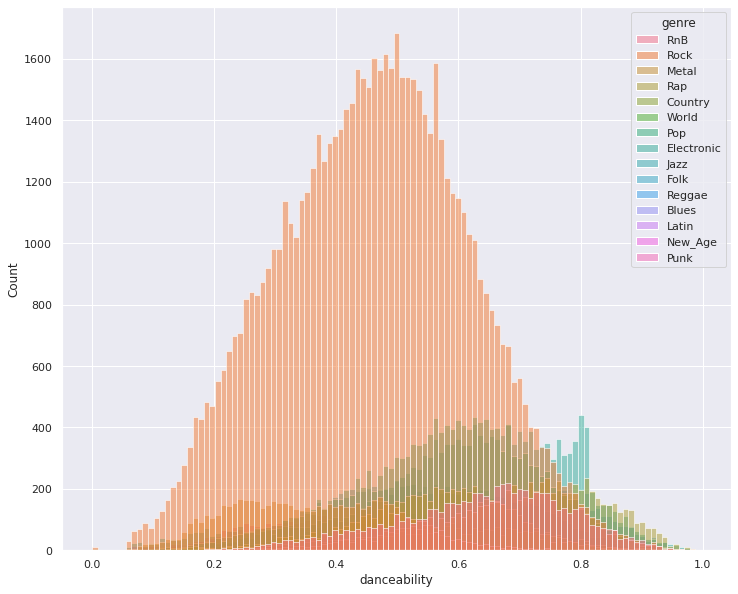
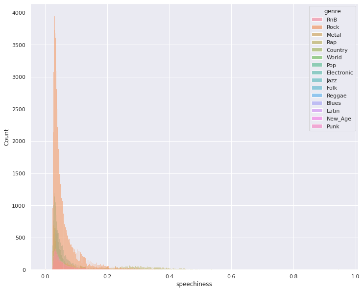
The above image shows how early in our data exploration process, we see different features having different predictability capabilities (forms in its distribution by genre that can provide useful information). We can additionally see again our data is inherently skewed towards the genre “Rock.” Finding ways to subsample datapoints of class Rock in our dataset is a method we hope to explore as a way to mitigate this issue.

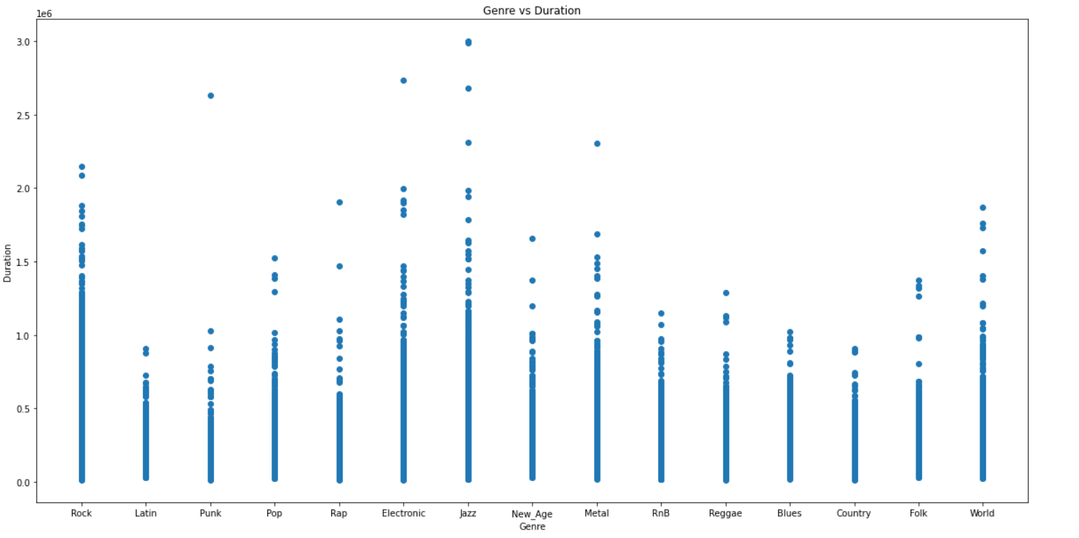
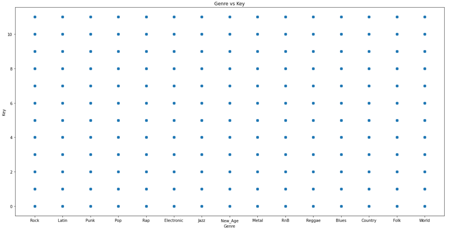
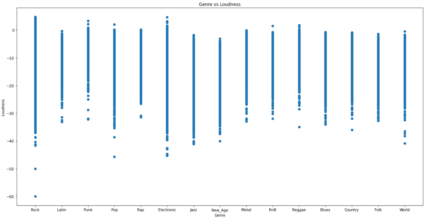
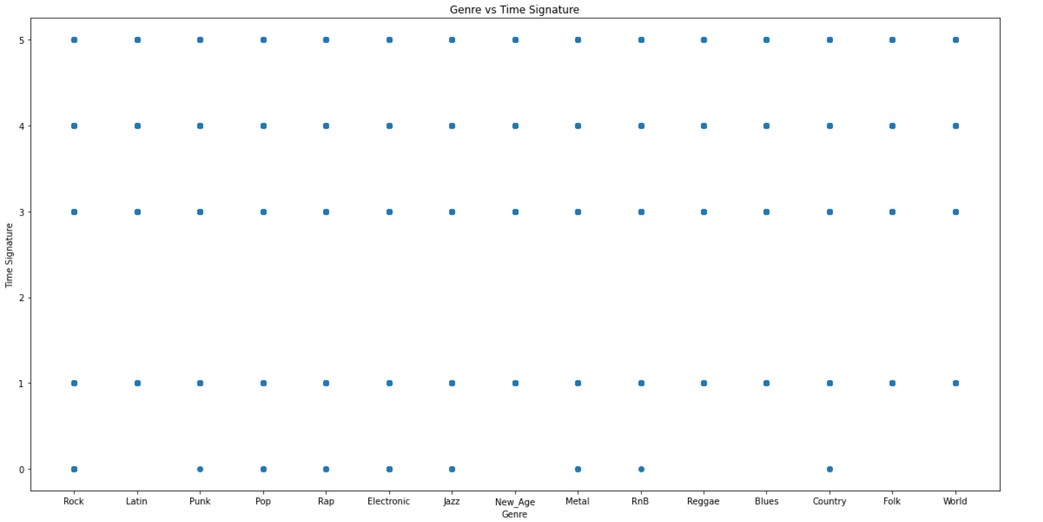
Included below are scatter plots of some of the audio features vs the genre label.

PCA and Dimensionality Reduction

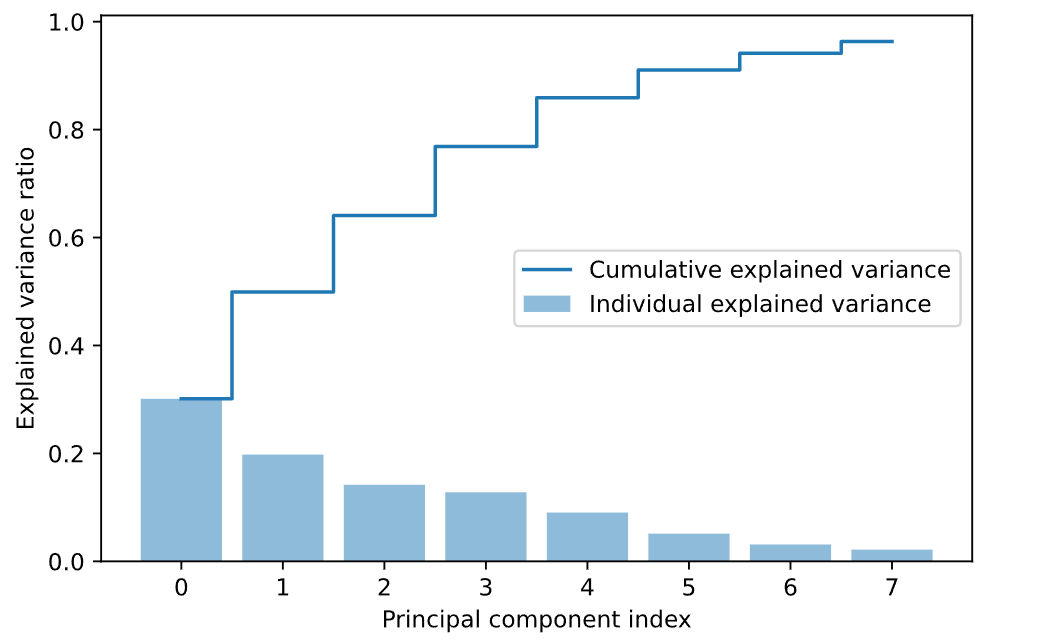
The original dataset that we created using information from Spotify had 13 features as explained previously. All the columns/attributes were considered as features except the columns containing song/track ids and the genre column, which we used as our label. Since this was a large dataset with several features, we used Principal Component Analysis (PCA) to reduce the dimensionality of the dataset which would potentially make it easier to work with. We chose a threshold of 0.95 for the explained variance ratio to keep only the most important features. This helped us get a transformed dataset with 8 components.

The figure below shows the explained variance ratio of each of the PCA components.

Final Updates

Also shown below is an interactive plot for PCA with 2 components. It shows the distribution of the data and gives us an idea of how the data is distributed. The clusters are taken from our K-Means output.

Supervised Learning Task: Genre Classification

Overall Results

Classifier	Accuracy	Precision	Recall	F1 Score
Logistic Regression Classifier (Original)	0.465	0.363	0.464	0.363
Logistic Regression Classifier (Balanced)	0.304	0.275	0.307	0.276
Decision Tree Classifier (Original)	0.314	0.319	0.314	0.316
Decision Tree Classifier (Balanced)	0.205	0.200	0.198	0.199
Random Forest Classifier (Original)	0.468	0.396	0.468	0.395
Random Forest Classifier (Balanced)	0.309	0.288	0.309	0.294
Neural Network Classifier (Original)	0.488	0.376	0.488	0.392
Neural Network Classifier (Balanced)	0.386	0.446	0.386	0.381
Gaussian Naive Bayes (Original)	0.377	0.421	0.377	0.381
Gaussian Naive Bayes (Balanced)	0.272	0.441	0.273	0.252
SVMs Classifier (Original)	0.481	0.347	0.482	0.365
SVMs Classifier (Balanced)	0.387	0.427	0.387	0.364

Original vs. Balanced Dataset Results

Final Updates

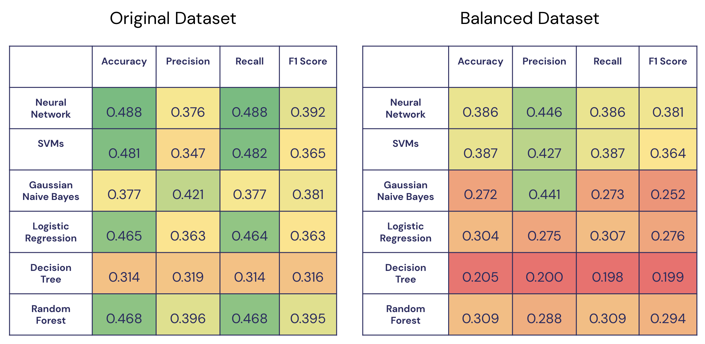
Overall, we see the highest accuracy from our original Neural Network model and the highest F1 score from our original Random Forest model. Additionally, we can see higher values for all 4 metrics in our original dataset over our balanced dataset. In the future, we are interested in finding other ways of balancing our dataset, such as using focal loss.

Logistic Regression Classifier

Original Dataset

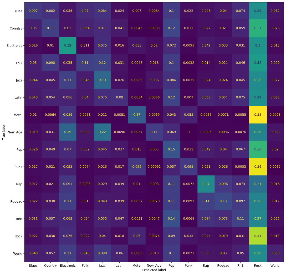
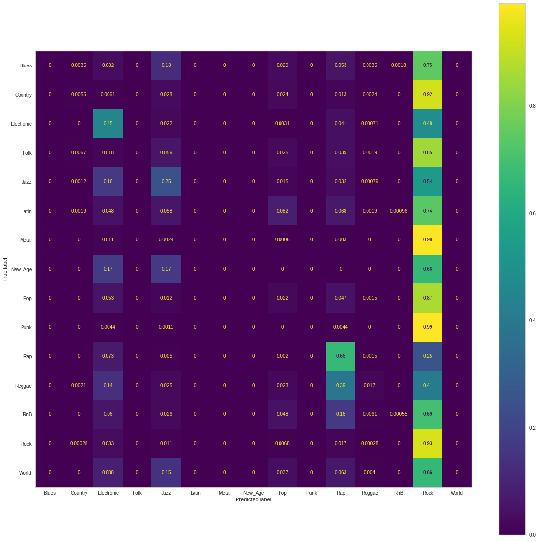
Using a Logistic Regression classifier, we were able to achieve 46% accuracy for classifying songs in each of the 15 genre classes. The following figure is a normalized confusion matrix for our Logistic Regression classifier.

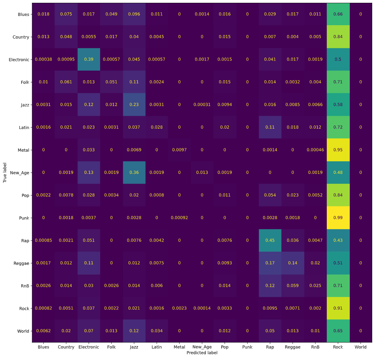
We noticed that rather than having high values along the diagonal, as we would have liked, we had a rather high number of songs being classified as Rock regardless of the true genre. As mentioned in our Dataset Exploration section, our dataset is heavily skewed towards Rock songs. Thus, our normalized confusion matrix for the Logistic Regression classifier shows that most songs were classified as Rock songs.

Balanced Dataset

To remedy the issue above, we balanced our dataset by finding the lowest genre count, which was 2,141 songs in the New Age genre, and using only that many songs from each genre; in doing so, we ensured an equal number of songs in each genre label. The resulting dataset had 2,141 songs for each of the 15 genres, so it had a total of 32,115 datapoints.

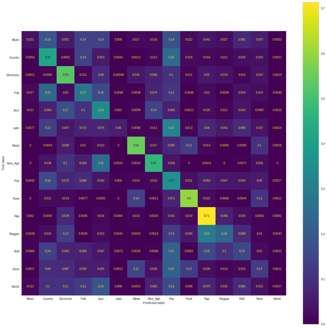
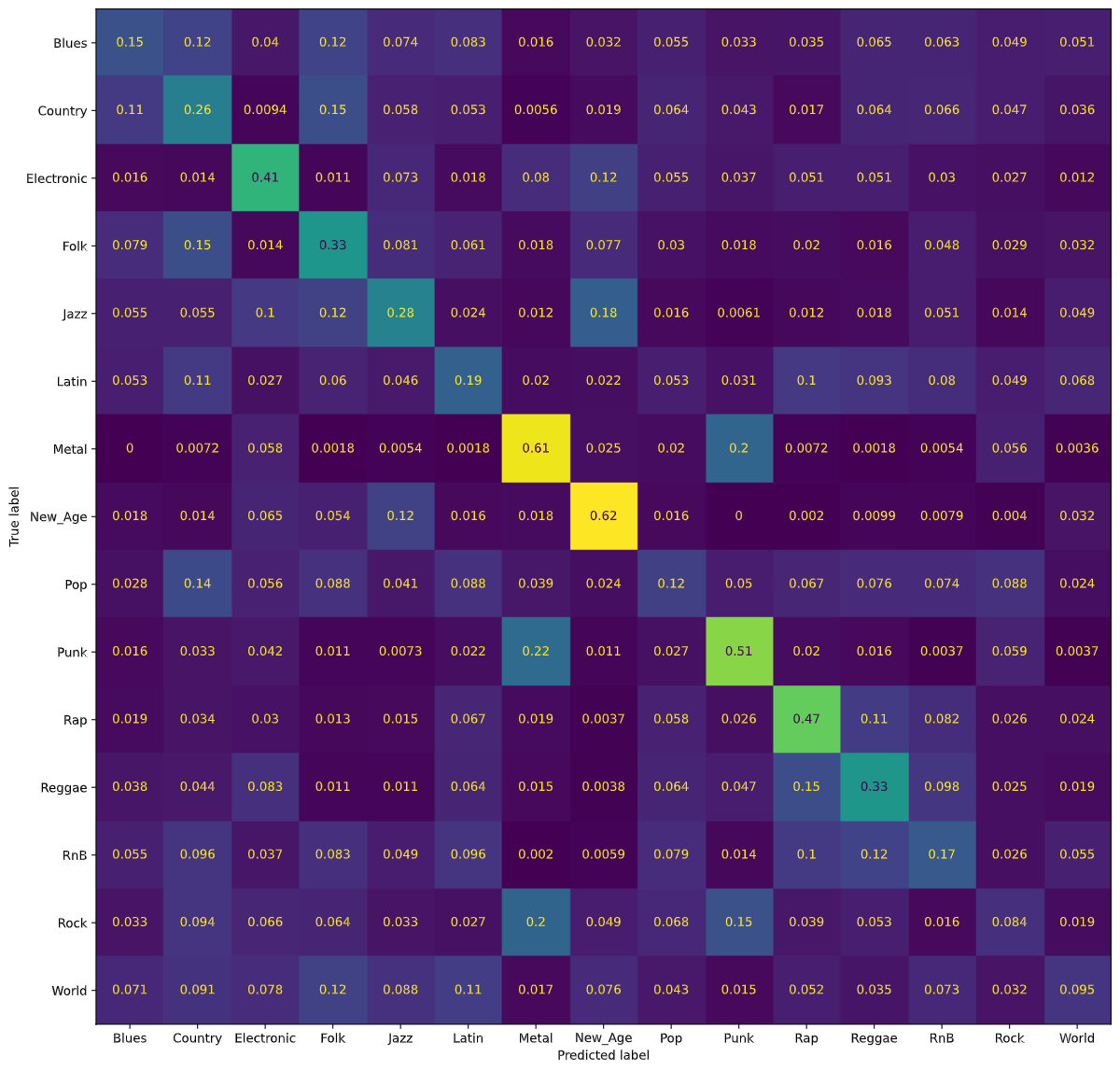
Using a Logistic Regression classifier with the balanced dataset, we were able to achieve 30% accuracy for classifying songs in each of the 15 genre classes. Notice that the accuracy of our Logistic Regression classifier went down from 46% to 30%. Despite this loss, we believe our new results are better, as the initial 46% accuracy may have been largely due to the fact that the classifier predicted that most songs were Rock songs and ended up being fairly accurate since an overwhelming proportion of the songs were in fact Rock songs. Even with the lower accuracy, our model still performs better than guessing genre at random, which would be roughly 1/15 = 6.6% accuracy. The following figure is a normalized confusion matrix for our Logistic Regression classifier with the balanced dataset.

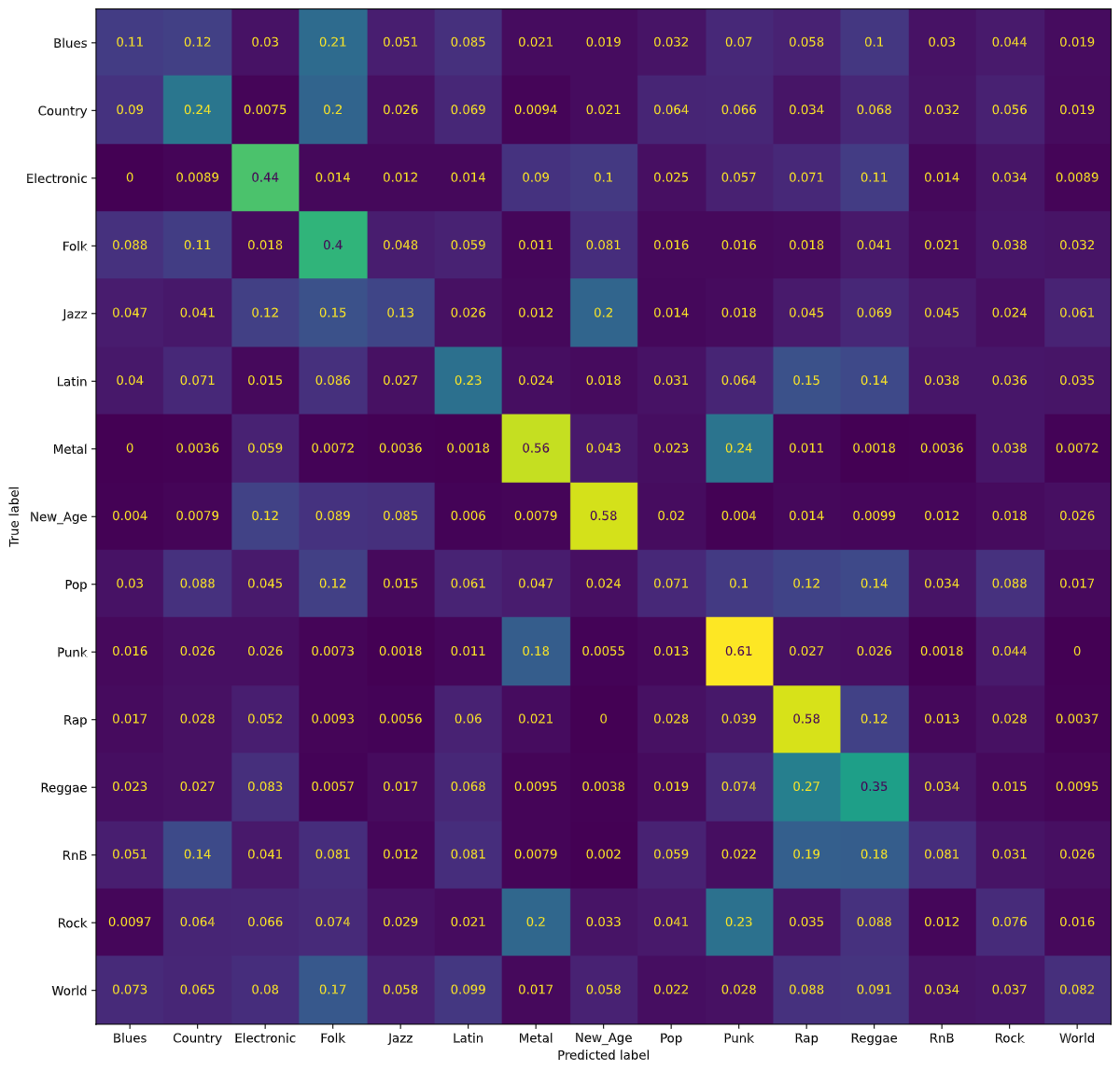
Notice that now, the values on the diagonal are much higher, signifying the model predicting the correct genre more often. Additionally, we are able to gain insights into which genres pairs that the model has trouble distinguishing. For example, the model has learned of similarities between the genre pairs Reggae/Rap, Metal/Punk, and Rock/Punk; these results are promising, as all three pairs of genres often have a large amount of musical overlap.

Decision Tree Classifier

Original Dataset

Using a Decision Tree classifier, we were able to achieve 31% accuracy for classifying songs in each of the 15 genre classes. The following figure is a normalized confusion matrix for our Decision Tree classifier.

We noticed that rather than having high values along the diagonal, as we would have liked, we had a rather high number of songs being classified as Rock regardless of the true genre. As mentioned in our Dataset Exploration section, our dataset is heavily skewed towards Rock songs. Thus, our normalized confusion matrix for the Decision Tree classifier also classifies most songs as Rock songs.

Balanced Dataset

As with the Logistic Regression classifier, we tried running the model again after balancing our dataset. Using a Decision Tree classifier with the balanced dataset, we were able to achieve 20% accuracy for classifying songs in each of the 15 genre classes. Again, notice that the accuracy of our Decision Tree classifier has gone down from 31% to 20%. Similar to Logistic Regression, we believe the results from the Decision Tree classifier are largely due to the fact that the classifier predicted most songs were Rock songs and ended up being correct since an overwhelming proportion of the songs were Rock songs. The following figure is a normalized confusion matrix for our Decision Tree classifier with the balanced dataset.

Notice that now, the values on the diagonal are much higher, signifying the model predicting the correct genre more often. Additionally, we are able to gain insights into which genres pairs that the model has trouble distinguishing. For example, the model has learned of similarities between the genre pairs Metal/Punk, Rock/Punk, and Country/Folk; these results are promising, as all three pairs of genres often have a large amount of musical overlap.

Neural Network

Results and Discussion

Another model which was saw as one that could have potential success was Neural Network model. We began with a transformation of our features and labels. Prior to running PCA, we started by transforming our features towards a multivariate normal distribution utilizing sklearn’s PowerTransformer implementation (with zero mean, unit standard deviation) as used in our other supervised models. While Box-Cox and Yeo-Johnson are both algorithms used for this transformation, we used Yeo-johnson due to its receptiveness of negative valued features. The preprocessing of labels consisted of encoding them into integers (Blues: 0, Country: 1, …, World: 15).

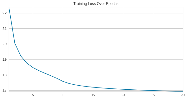
We began the exploration of this model type by having a simplistic structure to the network, a single hidden layer and an output layer of size number of classes with ReLU units being our activation function of choice throughout. The loss function we utilized was Cross Entropy Loss with SGD to optimize our parametres (with a learning rate of 0.0001 and momentum value of 0.9). We trained over a span of 30 epochs. We began the initial stages of model selection using K-Fold Cross Validation with the number of folds being used 4 and choosing models with the lowest average loss across folds. Additionally to see that our proposed models were not overfitting, we plotted the training and validation loss over multiple epochs (below image for when training on unbalanced dataset).

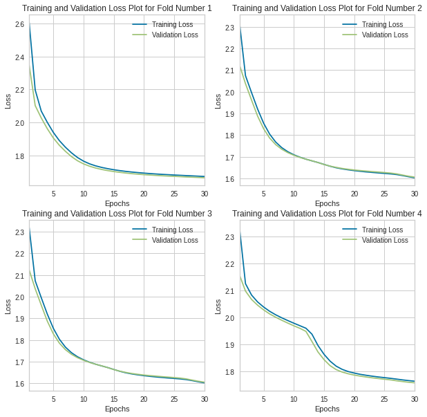
After tuning our parameters using the mentioned method, we then trained our chosen model and trained the model over the entire dataset. To provide as a sanity check that our model was in fact learning, we again plotted our loss curve and found the final training loss using Cross Entropy Loss of our model to be 1.693 when training on the unbalanced dataset.

Final Updates

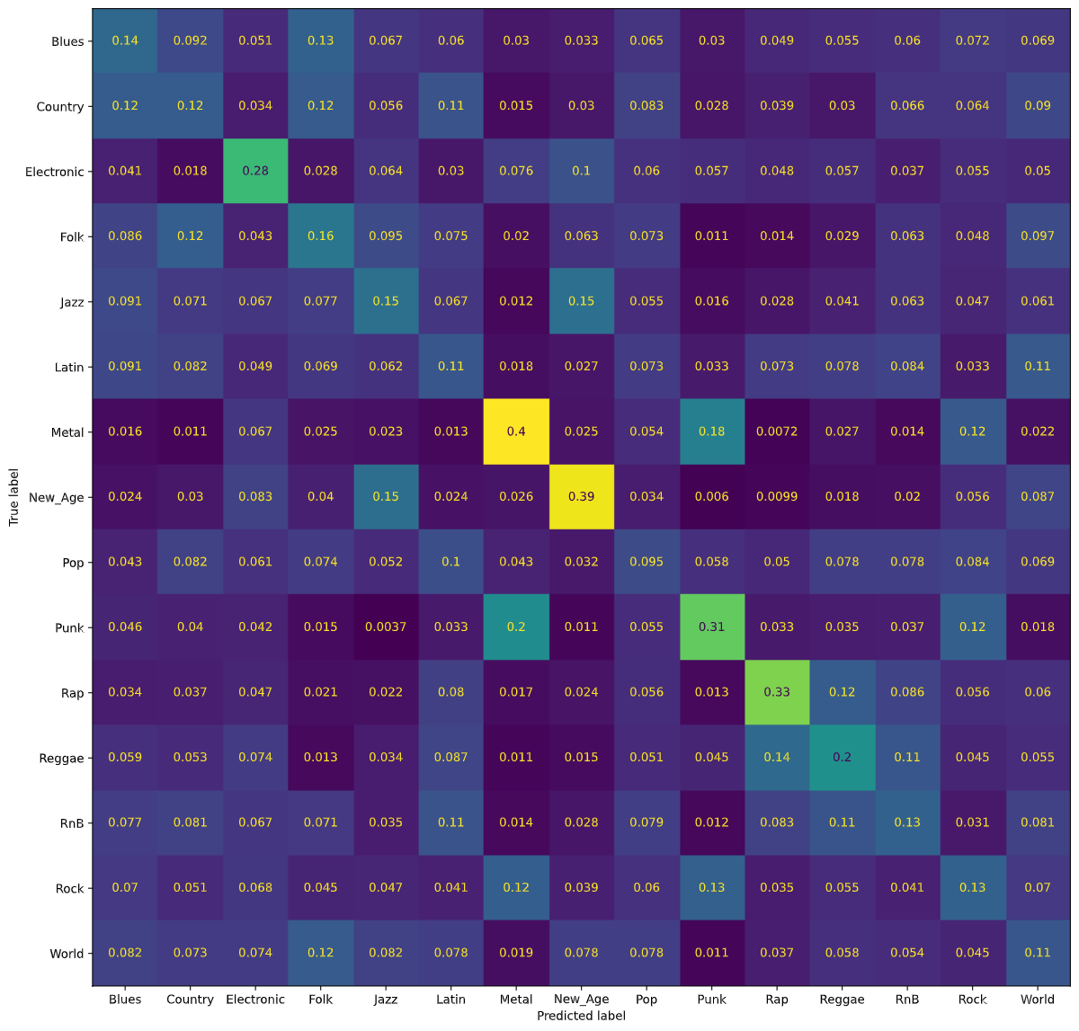
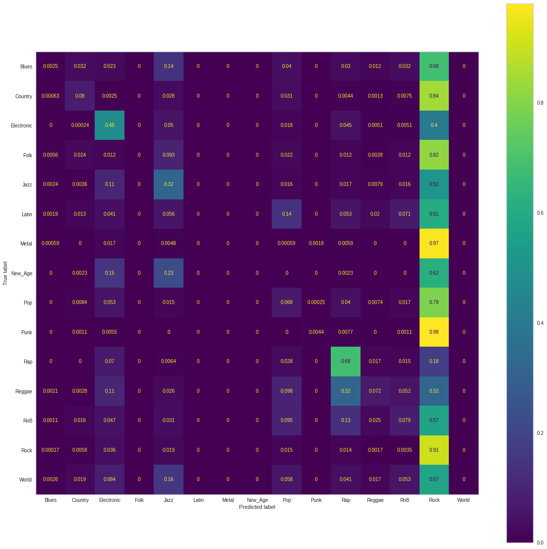
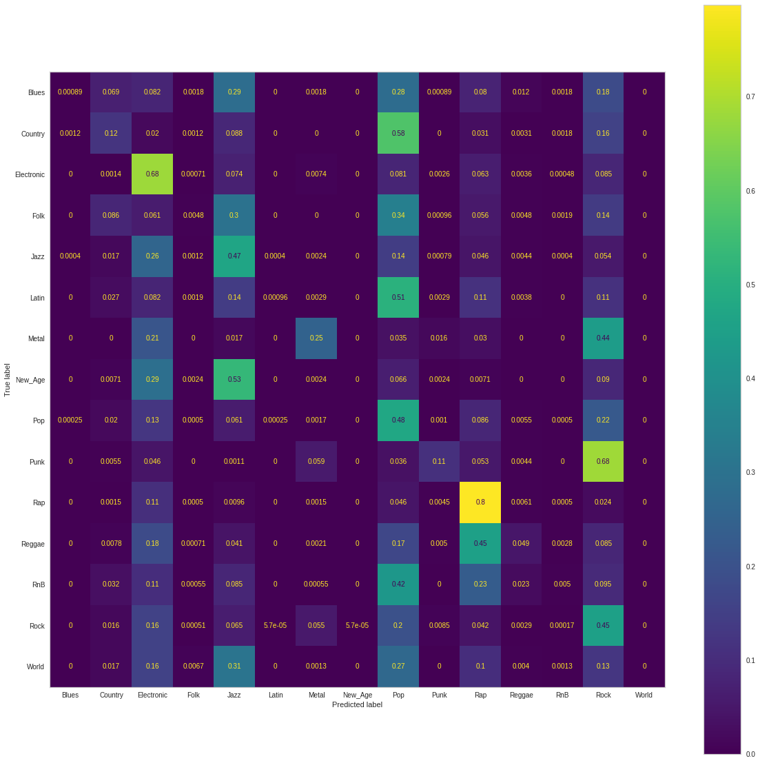
For our evaluation metrics to compare with success of other models, we use accuracy, precision, recall, and F1-score (given the nature of our dataset, accuracy will not hold as an all-encompassing metric). For the original imbalanced dataset, our model classifies the correct genre with accuracy 48.828%. In comparison, a naive approach of predicting all genres as “Rock,” would provide an accuracy of about 40%. The precision score, recall score and F1 score were calculated to be 0.376, 0.488, and 0.392 respectively. Below is the normalized Confusion Matrix when training on the unbalanced dataset:

When training this same model on our balanced dataset, we computed the the final training Cross Entropy Loss to be 1.862. Our achieved accuracy was 38.612%. The computed precision score, recall score, and F1 score were 0.446, 0.386, and 0.381. Below is the normalized Confusion Matrix when training on the balanced dataset:

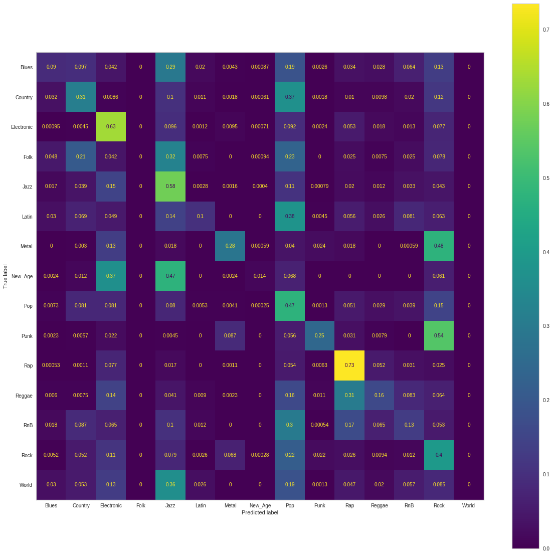
As exhibited in the prior supervised models, our accuracy suffered when balancing the dataset - the result of our model no longer overly predicting the dominant class Rock. When comparing the precision score, we see that our model trained on the balanced dataset is less likely to falsely classify a label as positive that is actually negative (i.e. the issue of labeling datapoints as Rock has been somewhat mitigated). However, we see that the recall score had gone down indicating our new models inability to find all positive examples. A worsened F1 score (a metric that is the harmonic mean of precision and recall) further indicates this inability, calling for further architecture search, hyperparameter tuning, etc.

Final Updates

Gaussian Naive Bayes Classfier

Another model we had trained and cursorily tuned was a GNB model. Regarding the performance the main interesting artifact was that although for our unbalanced dataset there was some reseblence of overly classifying songs as the dominant class “Rock,” the model was much more robust in learning classification predictions for classes that were in the minority. The following is the confusion matrix when trainined on the unbalanced dataset.

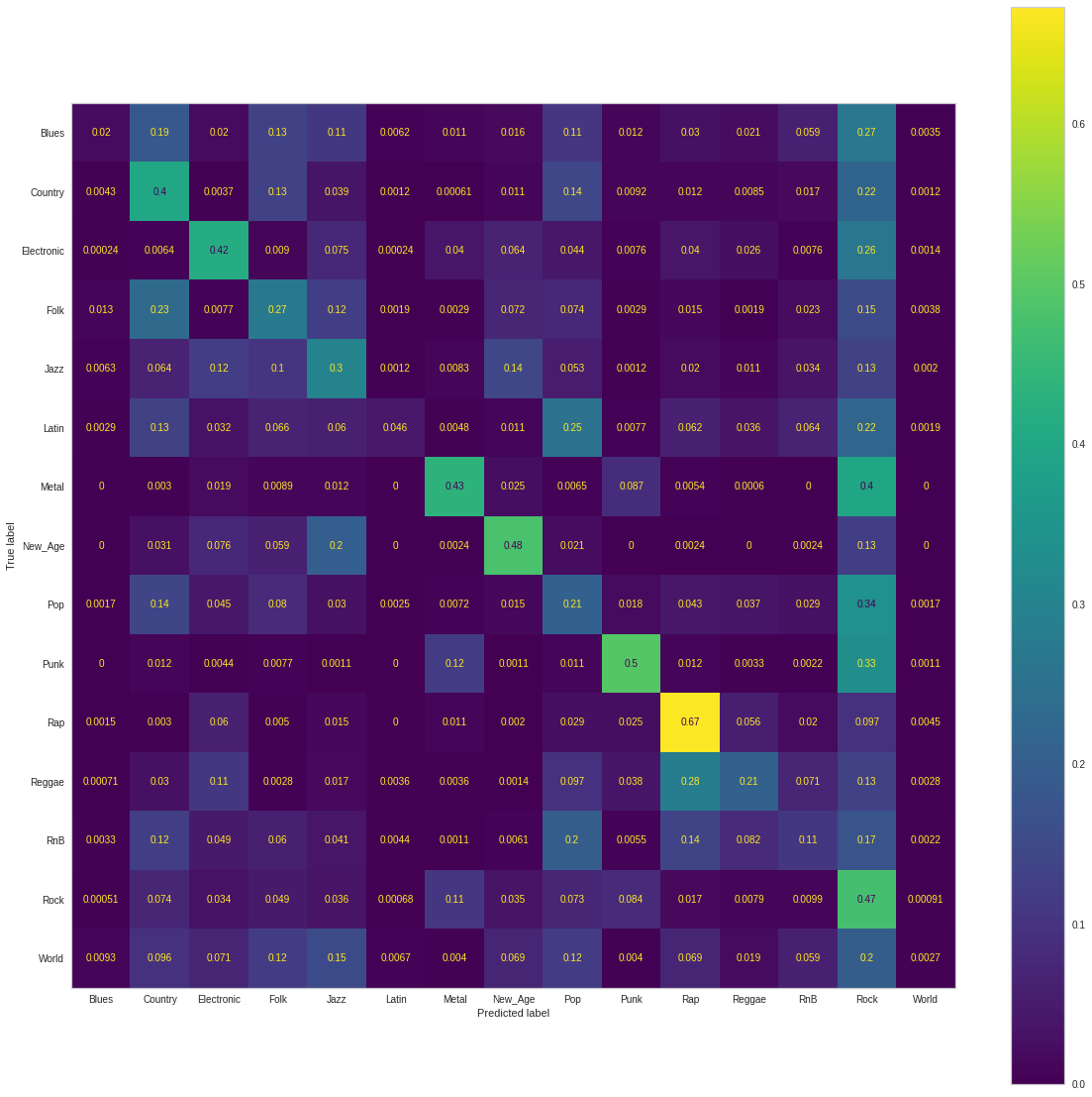
The accuracy we achieved with this classifier for the unbalanced dataset was .377. In comparison to other classifiers (e.g. NN, GNB), we see lower performance in this metric. However interestingly we se that the precision score was higher when compared to other models training on the unbalanced dataset. This indicates that this model displayed less false positives, resulting in an overall F1 Score (.381) comparable to other models after the balancing of the training data. Our recall score was somewhat less than models that simply learned to overly predict the dominant class given our models robustness to minority labels.

For our balanced training data, we erved the following Confusion Matrix:

Our accuracy (.272) suffered significantly while our precision (.441) similar to other models had gone up. However we not that this increase was not as drastic as other models. We can infer this is due to our GNBs initial success in this metric, the balancing of data’s improvement was less notable. As with the other models, for the balanced dataset we observed our F1 Score (.252) decrease due to reduction of True Positives identified by our model - seen by the reduction of our recall metric as well. We can attribute our models partial success to the preprocessing step of utilzing PCA components as features - ensuring that the Naive Bayes assumption holds for our model’s success.

Supper Vector Machines Classfier

Our group implemented SVMs as another model in our survey of supervised algorithms. The primarily focus for tuning this model was the regularization that we would utilize as well as the kernel method we would use (allowing our model to learn non-linearities). Similar to other models, we utilized cross validation to conduct grid search - evaluating validation performance for values of our regularizaiton parameter from 10^-3 to 10^3, an indicator of how large we want our margins. For lower values of C we prefer simpler SVM models and the opposite for higher values. Additionally we utilzed cross validation and determined the Radial Basis Function (RBF) Kernel as the most promising.

Here is the Confusion Matrix that we observed when training on Unbalanced data:

Performance wise, we see that it is quite similar to the neural network with relatively high accuracy (.481) and recall (.482) due to the model’s over-emphasis on “Rock” songs. The precision (.347) is relatively low due to the abundance of false positives for Rock songs. The F1 Score, a harmonic mean of precision and recall thus is hampered (.365)

Here is the Confusion Matrix that we observed when training on our Balanced dataset.

As observed prior, our model sacrafices accuracy (.387) and recall (.387) for increase ability for discriminating categories. Our precision rate (.426) thus goes up with less false positives. Due to the improvement in precision and regression with respect to recall, our F1 score for our model trainined on the balanced dataset remains relatively the same (.364).

Random Forest Classifier

Original Dataset

To improve upon our the results of our Decision Tree classifier, we decided to implement a Random Forest classifier as well.

Using a Random Forest classifier, we were able to achieve 46% accuracy for classifying songs in each of the 15 genre classes. The following figure is a normalized confusion matrix for our Decision Tree classifier.

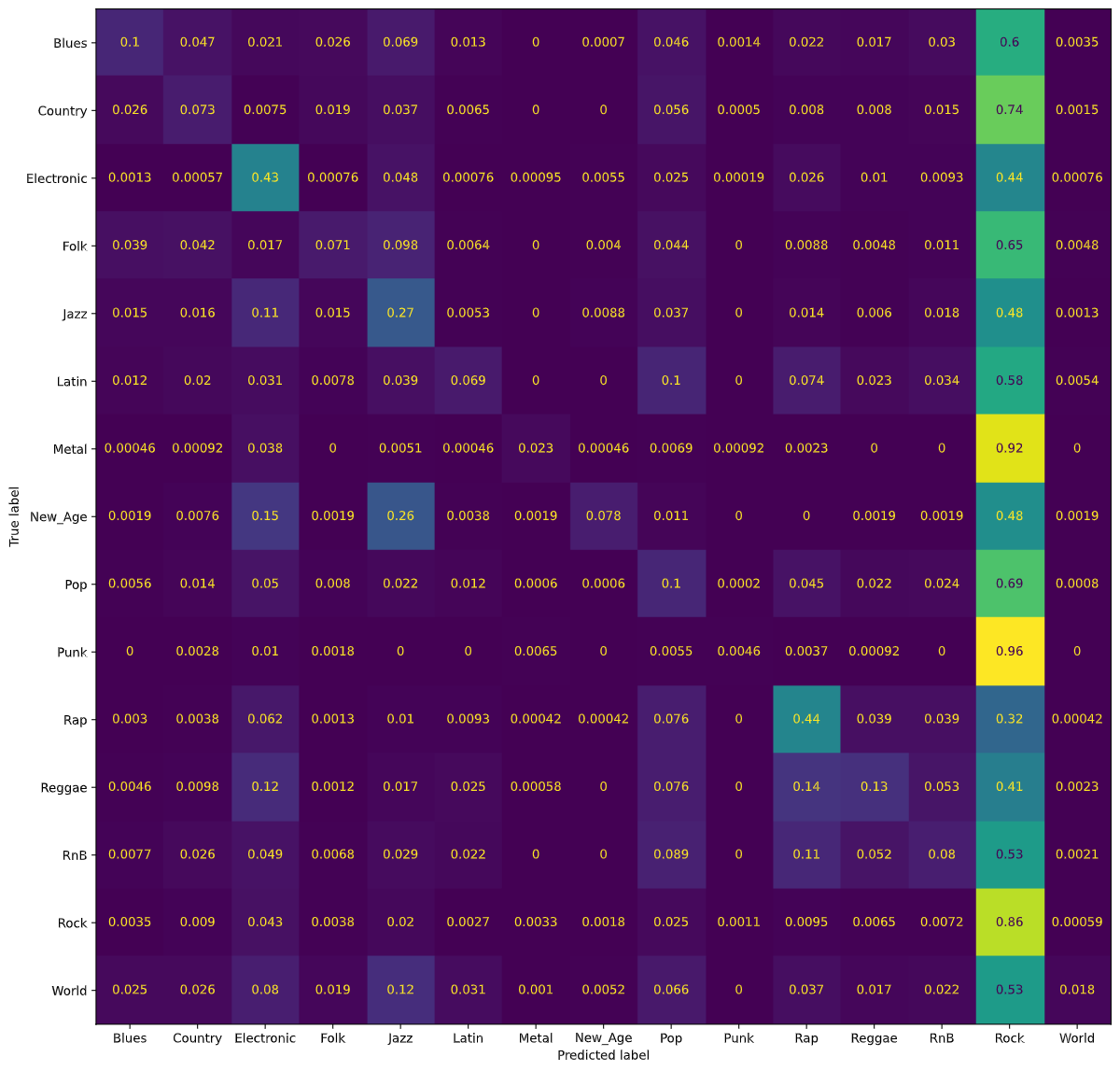
We noticed that rather than having high values along the diagonal, as we would have liked, we had a rather high number of songs being classified as Rock regardless of the true genre. As mentioned in our Dataset Exploration section, our dataset is heavily skewed towards Rock songs. Thus, our normalized confusion matrix for the Random Forest classifier also classifies most songs as Rock songs.

Balanced Dataset

We tried running the model again after balancing our dataset. Using a Random Forest classifier with the balanced dataset, we were able to achieve 30% accuracy for classifying songs in each of the 15 genre classes. Again, notice that the accuracy of our Random Forest classifier has gone down from 46% to 30%. Similar to Logistic Regression and Decision Tree, we believe the results from the Random Forest classifier are largely due to the fact that the classifier predicted most songs were Rock songs and ended up being correct since an overwhelming proportion of the songs were Rock songs. The following figure is a normalized confusion matrix for our Random Forest classifier with the balanced dataset.

Notice that now, the values on the diagonal are much higher, signifying the model predicting the correct genre more often. In contrast to the confusion matrices for Logistic Regression and Decision Tree, however, it is harder to see pairs of genres that are classified as similar from the results of our Random Forest classifier.

Unsupervised Learning Task: Song Clustering

The MusixMatch Dataset contained song lyrics in a bag of words format. We analyzed songs that were located both in the musiXmatch dataset and the original dataset we created from the MSD, Tagtraum labels, and Spotify features. From there, a dictionary was created with the word and word count listed for each track_id. Below is an illustration:

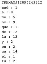
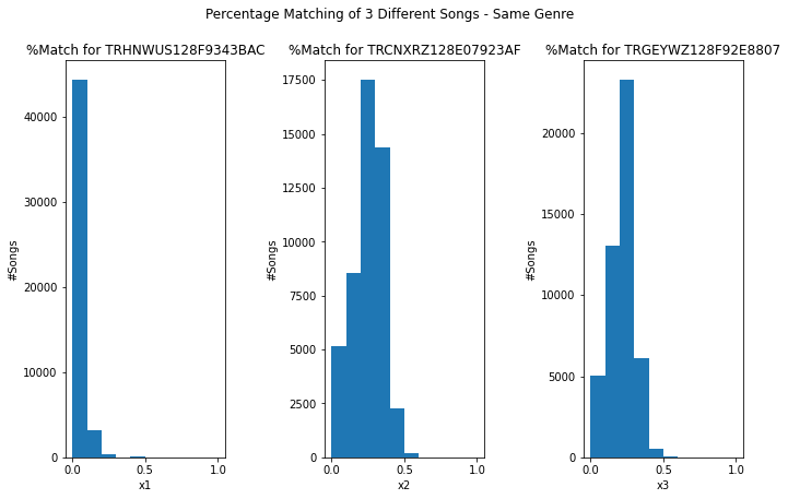
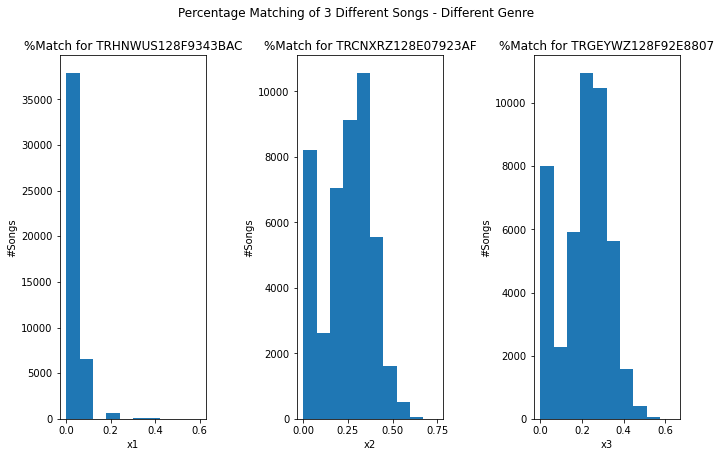
The dictionary contained 93,356 unique track_ids. From there, three random songs from our dictionary were chosen. Then, we compared the percent overlap between the unique words contained in the random song and those from another song in the dictionary. (Note that we only consider the individual words themselves, not their frequency of occurrence in the songs.) Percent overlap is calculated by comparing the number of shared words over the number of words documented in the random song. For example, if the two songs had six words in common and the random song had a total of ten unique words, then the percent overlap would be 60%, or 0.6.

We then decided to compare percent overlap values between songs that belong to the same/a different genre as/than the random song. Here are our results below:

Lyrics-Based Approach

Midterm update:

A future direction to pursue is to consider applying natural language processing models to our bags of words. As mentioned earlier in the report, we calculated similarity between songs using percent overlap. Since our objective is to find songs with overlap in lyrics, we can ignore songs from the dictionary that have little to no percent overlap. The downside to this metric of course is that the word count does not influence the percent overlap calculation. Two songs can for example contain similar sets of unique words, but may not be similar at all in terms of word count across this commonality.

The other issue is that even if we find songs with a high percent overlap with the common words and there are similar word count values across, we do not know the order in which the words appear in each of the respective songs.

A possible solution is to examine natural language processing techniques where the order of the words does not matter. We could use some kind of n-gram methods for example (i.e. like skip-gram, syntactic n-grams, etc). [8]

Final Updates

Preprocessing

The dataset described in the unsupervised task exploration section was used for the lyrics-based approach. Nevertheless, we did not find certain words such as articles and pronouns to be that significant in our analysis. Most every song would likely contain these words and the words themselves do not carry a lot of meaning. Therefore, we filtered out each of the songs’ bag of words using nltk’s stop words.

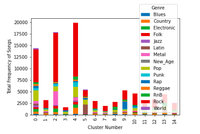
Clustering

In addition to seeing if song features correlated with genre, we also checked to see if a distinctive lyric-genre correlation existed. The goal of this analysis was to see if songs grouped together by similarity in lyrics can be mapped to the same genre. We used KMeans and created 15 clusters since we have 15 genres. Our results show that there does not appear to be a distinctive correlation. Therefore, this is an indicator that we can easily match users to a song from a different genre using similar lyrics.

Word2Vec Skip-Gram & TF-IDF

We decided to generate song recommendations based on two different models: Word2Vec and TF-IDF. Each model was tested for two different cases.

Case 1: Generate a random song and give ten song recommendations from a different genre

Case 2: Generate ten random songs and recommend a song

Note that the 2nd case is not genre-constrained. The same song (Case 1) and set of ten songs (Case 2) are tested against both models.

For the word2vec skip-gram model, we used the first 80% of the data to train the model and used the latter 20% as our test set. The different words have their own respective word representations. Therefore, we sum across each word contained in the bag of words (including repeats) to create a vector representation of the entire song.

From the test set, the algorithm picked out a random song. Then, it compared the chosen song against all of the other songs that are from a different genre. Cosine distance was used as our similarity metric, where the smalleer the value, the higher the similarity is between the two entities. The top ten recommendations and the single recommendation are given based on shortest distance.

Case 1 - Word2Vec:

Recommendation 1 : TRSPBAV128F427786A Recommendation 2 : TRQMQTZ128F92DC10A Recommendation 3 : TRWWJDX128F42818C7 Recommendation 4 : TRDMFZZ128F423D4B1 Recommendation 5 : TROLFDU12903CBDF36 Recommendation 6 : TRMJKMB12903CCDC79 Recommendation 7 : TRRWMRA128F92E3989 Recommendation 8 : TRIUNNK12903CCEAD0 Recommendation 9 : TRGIWUB128F1466D61 Recommendation 10 : TREFIVS12903D03ECF

Case 2 - Word2Vec

Recommendation: TRQNHFG128F932047D

Our TF-IDF model calculates a word significance weight for each unique word in the song based on 1) how frequently an the word shows up in the song and 2) how many songs its corresponding genre contain that lyric.Traditional TF-IDF are typically framed across the corpus as a whole, not the category to which the song belongs. Our goal was to find (different genres) recommended song(s) that had similar word significance weights as our random song(s). Like Word2Vec, we also used the cosine similarity metrics to compare songs. Below are the recommendations for each case.

Case 1 - TF-IDF

Recommendation 1 : TRDXRVT128E078EA86 Recommendation 2 : TRGDLQC128F4270523 Recommendation 3 : TRJSRWA128F92CD64C Recommendation 4 : TRSHBDG128F1493B34 Recommendation 5 : TRRKVTG128F4266634 Recommendation 6 : TRJSJXD128F1465C5E Recommendation 7 : TRULRPW128F92E7190 Recommendation 8 : TRUEHQP128F42647EF Recommendation 9 : TRVSWYO128E07963B5 Recommendation 10 : TRUJQWL128F4293557

Case 2 - TF-IDF

Recommendation: TRABMMM128F429199D

Since Word2Vec focuses on vectorization of individual words and TF-IDF is geared toward word significance, it is not all that surprising that the recommendations from the two models are completely different from one another. Judging which one is “better” depends perhaps on the users’ preferences. If they care that the two songs have a similar set of words with similar frequencies, then Word2Vec would be the more appropriate approach. Otherwise, if they want the songs to have similar enough lyrics but also hold the similar amount of relevance to their respective genres, then the TF-IDF method is more effective.

Spotify Features Approach

Clustering Evaluation

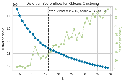
For our unsupervised data-exploration, we decided to cluster using K-Means and GMM. To decide the number of clusters we visualized various clustering evaluations to see how “good” our clustering was. For exploring the selection of number of clusters, we decided to train multiple K-Means (GMM excluded to reduce scope) and evaluated different K-values and provided associated visuals when clustering on the balanced and unbalanced dataset. For majority of our metrics, we compare clusters of size 2-30 for robustness. Finally although the Elbow Method suggested 15 was the optimal number of clusters for the algorithm (matching the 15 genre categories we had as ground truths), we prefered too use 5 clusters as suggested by the Silhouette method to further uncover relationships between genres and see if we can identify which genres the models groups together. The external clustering metrics, although interesting in exploration, did little in suggesting an optimal cluster for the balanced and unbalanced dataset.

Elbow Method

Unbalanced

For the unbalanced dataset, we interestingly see that the optimal number of clusters was 15, the number of genres we have in our dataset. Intuitively, we also see that as the number of clusters increase, so does the model fitting time.

Balanced

For the balanced dataset, we the optimal number of clusters being similar to that of the unbalanced dataset, 16. We see however that the distortion score, our objective function used to compare models is much higher. In brevity the distortion score is defined as the sum of squared distances of points to their associated center. We assume that this score is lower for the unbalanced dataset since the density of datapoints, or songs, associated to Rock must be quite high - skewing the overall average distortion score among other clusters.

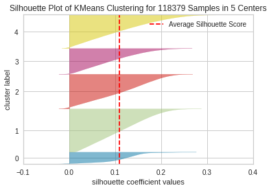
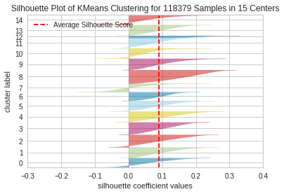
Silhouette Coefficient

Unbalanced

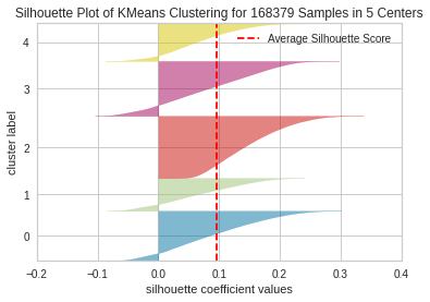
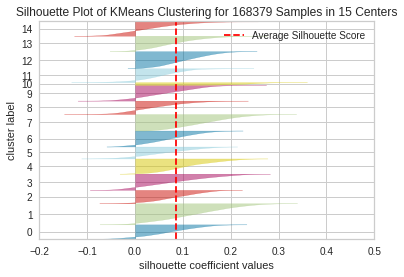
For visualization purposes, we see the Silhouette plot for a clustering using 5 centers and 15 centers. We consider an average Silhouette score as good for a given model depending on how close 1 it is (a normalized metric of the difference between the average intracluster distance and the mean nearest cluster distance). We additionally prefer the thickness associated to each cluster (indicating the proportion of points associated to each cluster) to be relatively uniform. We can see that there is a high degree of variation with respect to the clustering using 15 centers, suggesting the optimal number of clusters suggested by the elbow method is not optimal for this new metric.

Balanced

For the balanced dataset, the average score stayed relatively same for each cluster. An interesting thing to note however is the proportion of songs had been redistributed and looked to be much more uniform for the clustering with 5 centers (apart from the final cluster). The visual also helps give insight as to how certain points severely penalizes and rewards the average score depending on the placement within its associated cluster and with relation to other clusters.

External Measures : FMS Score, V-Measure Score, Rand Score

Unbalanced

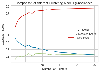
To utilize having ground truth labels for each associated song, we saw that utilizing external measures might be a fruitful source of exploration. To reduce scope, we focused on 3 pairwise metrics, FMS Score, V-Measure Score and Rand Score. FMS Score we thought to be useful due to its integration of pairwise precision and recall (measuring the geometric mean of the two). The Rand Score we thought we would be similarly useful as it helps visualize the true positive and true negatives produced among pairs. Lastly the V-Measure Score was another metric that may be useful given the information it gives regarding the homogenity (the extent to which each cluster is comprised of a single or few labels) and completeness (the extent that all points associate to a class is fitted in the same cluster).

For good clustering we expecta V-Measure approaching 1, a Rand score close to 1 and FMS score close to 1.

For the clustering on the unbalanced dataset, we can see first that the Rand Score seems to arbitrarily improve as the number of clusters increases. Interestingly we see that the V-Measure score seems to remain constant among the clusterings. We hypothesize this as to the trade off of improving homogenity as we increase the number of clusters (we can arbitrarily create groups that encompases subclusters of labels) and worsening the completeness (points associated to a particular label are more likely to be partitioned. Lastly for the FMS Score we see that this metric worsens as we increase the number of clusters.

Balanced

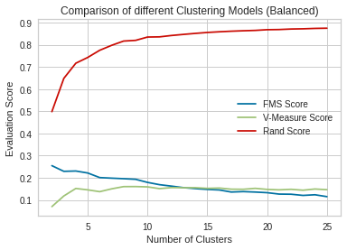
Similar for the case of clustering with the unbalanced dataset, we can see that the Rand Score seems to arbitrarily improve as the number of clusters increases. We additionally see that the V-Measure score tends to stay consistent as we increase the number of clusterings. Lastly, we again see that the FMS score worsens as we increase the number of clusters.

K-Means

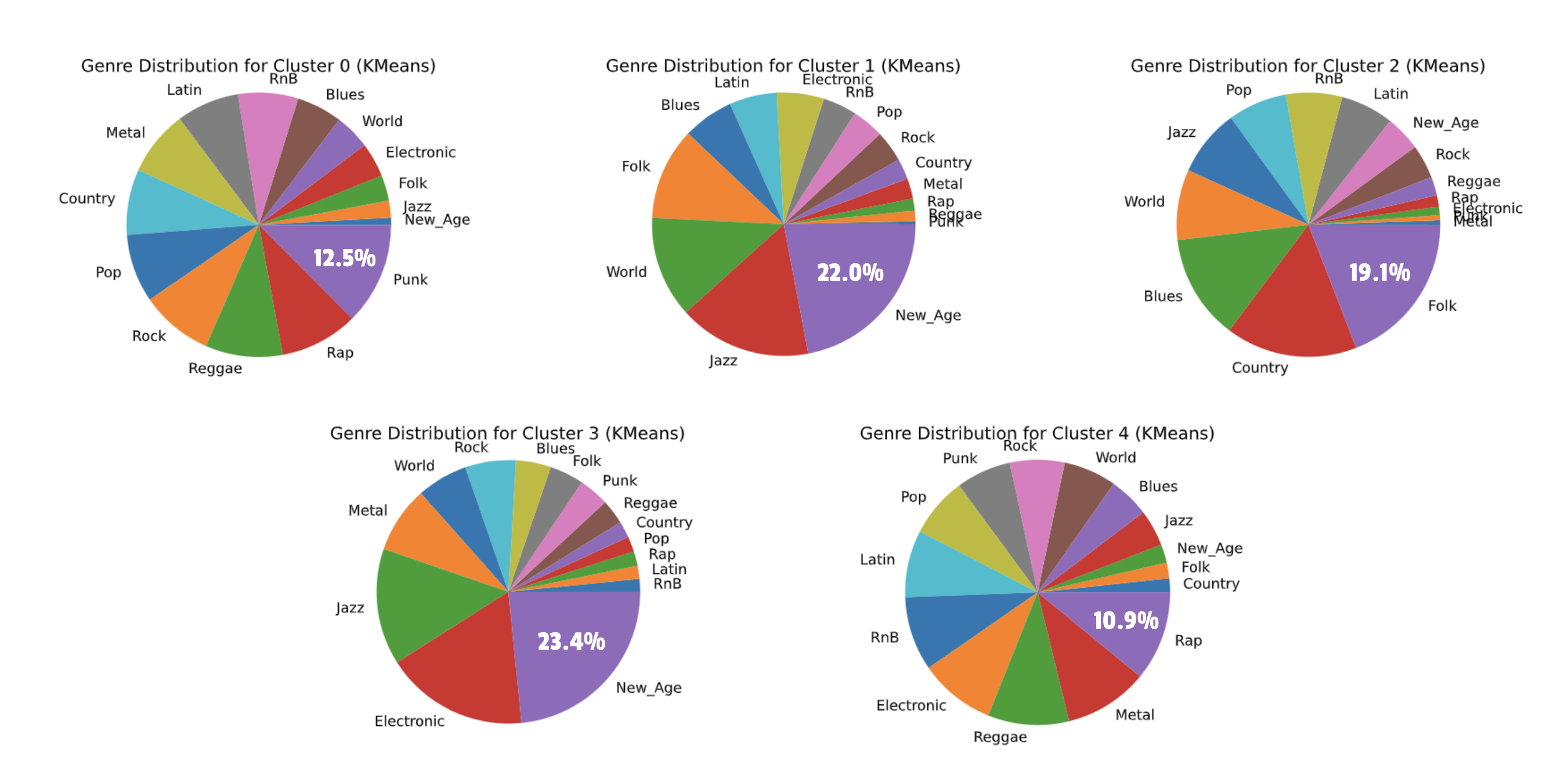
The following pie charts show the distribution of genres in each of the 5 clusters from our K-Means clustering. Notice the labels for the purity of each of these clusters, ranging from 10.9% to 23.4% purity.

Gaussian Mixture Model

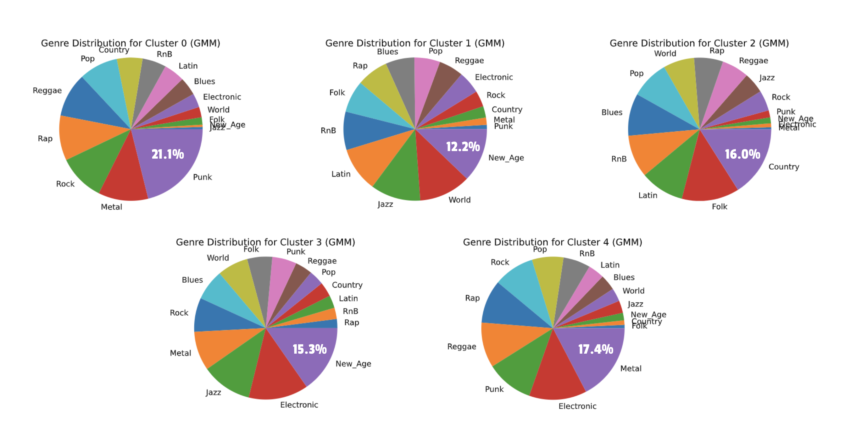
The following pie charts show the distribution of genres in each of the 5 clusters from our GMM clustering. Notice the labels for the purity of each of these clusters, ranging from 12.2% to 21.1% purity. In K-Means and GMM, you can see that Punk and Metal were highly clustered together, as were Country and Folk. These pairings are expected since these genres are highly related.

Genreless Music Recommendation System

In the final phase of the project, we decided to build a music recommendation system. As stated in our proposal, we wanted to devise a system that recommends similar songs irrespective of genre. Our hypothesis was that users would like their recommendations to be similar to the songs they like. Genre does not play a very important role. In fact, all our exploratory algorithms showed that the audio features have little correlation with genre, which explains why predicting genre using these features yields poor results. Compared to audio features such as acousticness, energy, tempo, valence, etc., genre is a highly subjective and loose categorical feature. Songs in different genres may end up being closer to one another (with respect to their audio features) and our hypothesis was that users would prefer to listen to these similar songs even if they were in a different genre.

We used a content-based recommendation system where we take song inputs from the user, find the mean vector of those songs and then recommend songs that are closest to that mean vector. There are other recommendation systems such as collaborative filtering but since we did not have any user data (such as ratings or reviews) we decided to use the content-based approach. Following is a step-by-step description of the algorithm:

1. Take song inputs from the user. Any song present on Spotify may be entered as input. However, our recommendations are limited to the songs available in our final cleaned Million Song Dataset (~210k tracks). The user may specify as many songs as they like in the form of a JSON list with the following keys:
   • Song name
   • Release year
   • Spotify track ID
2. For the input list, find the mean vector. This vector is basically a mean of the audio features of the songs (using the features described in Dataset Collection). We call this the song center.

3. Find the n-closest datapoints to the song center and recommend the songs corresponding to those datapoints to the user. By default, we recommend n_songs = 10 but it can be passed as a parameter to our recommendation function to tweak the number of recommendations as desired. To compute the closeness of the datapoints, we used the cosine distance, which can be defined as :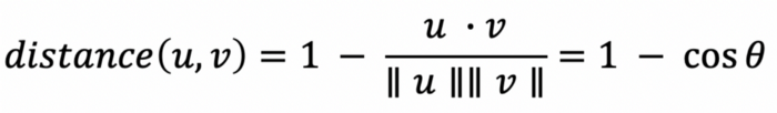
   We used the cdist function from the scipy library to compute this.

4. Return the recommendations to the user formatted as song name and artist. We ensure that the recommendations do not contain any songs from the input list.

Output and observations

We observed our recommendation system to perform fairly well. Our team members tested out the recommendation system with a variety of inputs and the results were deemed relevant and satisfactory. In general, we observed that the recommended songs were quite similar in audio features to the songs provided as inputs, which was expected of course. So, if an user were to input a list of songs with high-tempo and lots of guitar and drum riffs, they would receive recommendations for songs with a similar high energy and heavy usage guitars and drums. Using a list of more acoustic songs resulted in acoustic recommendations. If the input songs had only music but no vocals, the output recommendations would also be musical pieces with little to no vocals. One interesting case was when we used a long 30-min song as an input. The recommendation system returned another song which was 20-min long, indicating that the system was able to learn certain patterns from the input song, identify similar patterns from the dataset and recommend similar songs to the users.

Included below are two screenshots which shows the recommendations for users with different tastes in songs as input. As you can see, the recommendations are similar to the input songs (You can listen to these songs on Spotify to verify!)

Recommendation for a user with who enjoys rock and similar kinds of music. The recommendations reflect an average of the audio features of the inputs.

Recommendation for a user who only provides one song as input. n_songs has also been chosen as 5 for this example.

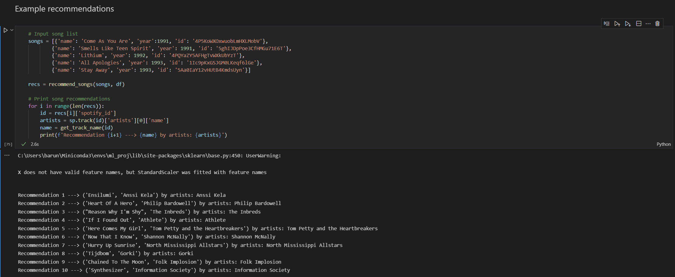
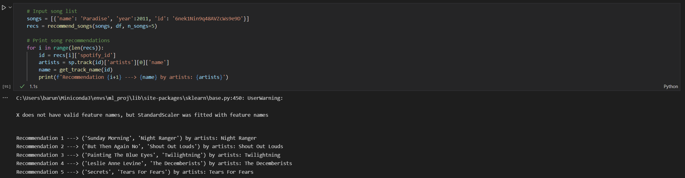
To the best of our knowledge, there was no significant effect of the number of songs provided as input.

Challenges faced

1. The dataset is heavily skewed towards Rock songs, which are the overwhelming majority of data points in the dataset. This makes it difficult to accurately predict the genre of a song and we had to perform standardization and balancing of the dataset to make it more accurate. However, balancing results in discarding a lot of information. Hence, the sheer number of Rock songs in the dataset still represents a challenge for analysis.
2. Our recommendation system is limited by the number of songs available in the dataset. This means we were unable to recommend songs that might have been more relevant but were not present in the dataset. There was no way to counter this problem and this is a known flaw in the system that we recognize.
3. We did not detect any effect of the number of songs provided as input to the recommendation system. However, since we chose to simply average the audio features of the input song list, it is possible that in the case when the inputs are widely different, the average might point to a completely different song, which is not very accurate. Simply put, an average smoothes over the differences and our system does not have a way to fine-tune the recommendations based on the input songs. For instance, if a user chooses as input a heavy drum-based song and another soft instrumental song, their average vector might be a song with few vocals and a moderate amount of drumbeats (i.e., an average of the two inputs), which might sound like a pop song. This new song might not be very relevant for the user, who might intuituvely have expected the system to provide more songs that were similar to his taste (i.e., more instrumental songs and more drum-based songs, but not a mix of both).

Future scope

While we are pleased with our project so far, we also had a few ideas on how we could improve certain parts. While time constraints prevented us from exploring these further, we believe these are steps that could be taken to improve the project’s performance in the future.

1. One potential improvement is to balance the dataset so that our algorithms and recommendations are not skewed by the overwhelming majority of rock songs in the dataset. One possible way to do this might be by exploring relevant metrics such as focal loss.
2. Another potential improvement is to use a more sophisticated recommendation system that can preserve the individuality of the input. This would solve the problem of averaging the audio features of the input songs. Perhaps we could explore different weighting strategies for each of the inputs if they differ widely from each other, or we could have a threshold and if the input songs differ by more than that threshold, we could consider that a separate category and recommend songs from that category to the user.
3. We could explore ways to combine the lyrics and audio features to come up with a more robust and accurate recommendation system. This could yield better genreless results since our experiments showed that both lyrics and audio features had low correlatation to the genre.
4. There’s always a few changes to the lyrics-based approach that could be investigated. For example, we could into actually using the entirety of the corpus for TF-IDF analysis and see how the recommendations compare to the existing TF-IDF and Word2Vec models. We could also change the train-test percentage on Word2Vec to see how that influences the results. Finally, we could even modify which stop words are filtered (and perhaps add additional words to the list of stop words) and see how all analyses succeeding that get affected.

References

[1] J. Kristensen, “The rise of the genre-less music fan,” RSS, 22-Mar-2021. [Online]. Available: https://www.audiencerepublic.com/blog/the-rise-of-the-genre-less-music-fan. [Accessed: 21-Feb-2022].

[2] H. Datta, G. Knox, and B. J. Bronnenberg, “Changing their tune: How consumers’ adoption of online streaming affects music consumption and discovery,” Marketing Science, vol. 37, no. 1, pp. 5–21, 2018.

[3] E. Canty, “The effect different genres of music can have on your mind, body, and community.,” Upworthy, 02-Feb-2022. [Online]. Available: https://www.upworthy.com/the-effect-different-genres-of-music-can-have-on-your-mind-body-and-community. [Accessed: 21-Feb-2022].

[4] Adiyansjah, A. A. Gunawan, and D. Suhartono, “Music recommender system based on genre using convolutional recurrent neural networks,” Procedia Computer Science, vol. 157, pp. 99–109, 2019.

[5] K. Benzi, V. Kalofolias, X. Bresson, and P. Vandergheynst, “Song recommendation with non-negative matrix factorization and graph total variation,” 2016 IEEE International Conference on Acoustics, Speech and Signal Processing (ICASSP), 2016.

[6] M. Vystrčilová and L. Peška, “Lyrics or audio for music recommendation?,” Proceedings of the 10th International Conference on Web Intelligence, Mining and Semantics, 2020.

[7] S. Rawat, “Music genre classification using machine learning,” Analytics Steps. [Online]. Available: https://www.analyticssteps.com/blogs/music-genre-classification-using-machine-learning. [Accessed: 21-Feb-2022].

[8] D. Jurafsky and J.H. Martin, “N-gram Language Models,” Stanford University. [Online]. Available: https://web.stanford.edu/~jurafsky/slp3/3.pdf. [Accessed: 04-April-2022].